RVEA
Reference vectors divide objective space, and angle-penalized distance balances convergence and diversity during selection. Vector adaptation accounts for objective-space scales [1].
Goal: run the stable public API in VAMOS 1.4.0, interpret its returned population, and identify which settings control this mechanism.
Capability matrix · Exact configuration reference · Setup and recorded evidence
Run the example
Prerequisite: complete T01 and the coverage setup. The protocol uses DTLZ2, 12 real variables, 3 objectives, 10 reference vectors and population 10; 400 evaluations; NumPy; seed 42. Initial evaluations count towards the budget. Settings are illustrative, not tuned.
python rvea.py
python rvea.py --output rvea-local.svg
The second command reruns the same protocol and requires Matplotlib. Use a new filename.
Complete runnable script
"""Verified VAMOS 1.4.0 lesson: rvea. See coverage-setup for dependencies."""


def execute_example(problem, algorithm, config, budget, seed=42, engine="numpy"):
    import numpy as np

    from vamos import OptimizationResult, optimize

    result = optimize(problem, algorithm=algorithm, algorithm_config=config, max_evaluations=budget, seed=seed, engine=engine)
    G = result.data.get("G")
    if getattr(problem, "n_constraints", 0) and G is None:
        raise ValueError("Declared constraints are missing from the returned result.")
    feasible_rows = np.arange(len(result.F)) if G is None else np.flatnonzero(np.all(G <= 0, axis=1))
    if len(feasible_rows):
        feasible = OptimizationResult({"X": result.X[feasible_rows], "F": result.F[feasible_rows]})
        front, local = feasible.front(return_indices=True)
        front_rows = feasible_rows[local]
    else:
        front, front_rows = np.empty((0, problem.n_obj)), np.empty(0, dtype=int)
    print(f"Algorithm: {algorithm}; encoding: {problem.encoding}; backend: {engine}; seed: {seed}")
    print(f"Returned X: {result.X.shape}; F: {result.F.shape}; result mode: population")
    print(f"Feasible rows: {len(feasible_rows)}/{len(result.F)}; feasible non-dominated rows: {len(front)}")
    print(f"Evaluations: {result.data['evaluations']}")
    return {
        "problem": problem,
        "algorithm": algorithm,
        "config": config,
        "result": result,
        "feasible_rows": feasible_rows,
        "front": front,
        "front_rows": front_rows,
    }


def run_rvea(budget=400):
    from math import comb

    from vamos.algorithms import RVEAConfig
    from vamos.problems import DTLZ2

    problem = DTLZ2(n_var=12, n_obj=3)
    partitions = 3
    population = comb(partitions + problem.n_obj - 1, problem.n_obj - 1)
    config = (
        RVEAConfig.builder()
        .pop_size(population)
        .n_partitions(partitions)
        .alpha(2.0)
        .adapt_freq(0.1)
        .crossover("sbx", prob=1.0, eta=30.0)
        .mutation("pm", prob=1.0 / problem.n_var, eta=20.0)
        .constraint_mode("feasibility")
        .result_mode("population")
        .build()
    )
    return execute_example(problem, "rvea", config, budget)


def plot_example(data, output):
    from pathlib import Path

    import matplotlib

    matplotlib.use("Agg")
    import matplotlib.pyplot as plt
    import numpy as np

    output = Path(output)
    if output.exists():
        raise FileExistsError(f"Choose a new figure filename: {output}")
    if output.suffix.lower() != ".svg":
        raise ValueError("Use an .svg output filename.")
    f = data["result"].F
    with plt.rc_context({"svg.hashsalt": "vamos-coverage", "svg.fonttype": "none"}):
        fig = plt.figure(figsize=(7, 4.5), layout="constrained")
        if f.shape[1] == 3:
            ax = fig.add_subplot(projection="3d")
            ax.scatter(*f.T, c="#007f7a", s=22)
            ax.set(xlabel="f1", ylabel="f2", zlabel="f3")
            ax.set_box_aspect((1, 1, 0.85), zoom=0.85)
        else:
            ax = fig.add_subplot()
            ax.scatter(*f.T, c="#b6bec8", s=25, label="Returned population")
            if len(data["front"]):
                ax.scatter(*data["front"].T, c="#007f7a", s=30, label="Feasible non-dominated rows")
            labels = {
                "WeldedBeamDesignProblem": ("Cost (minimize)", "Deflection proxy (minimize)"),
                "FeatureSelectionProblem": ("Validation error (minimize)", "Feature count (minimize)"),
                "HyperparameterTuningProblem": ("Validation error (minimize)", "Complexity proxy (minimize)"),
            }
            xlabel, ylabel = labels.get(type(data["problem"]).__name__, ("f1 (minimize)", "f2 (minimize)"))
            ax.set(xlabel=xlabel, ylabel=ylabel)
            ax.legend()
        if data["problem"].__class__.__name__ in {"ZDT1", "ZDT1Problem"}:
            x = np.linspace(0, 1, 101)
            ax.plot(x, 1 - np.sqrt(x), "--", c="#7c8795", label="Analytical front")
            ax.legend()
        ax.set_title(f"{data['algorithm'].upper()} · {data['result'].data['evaluations']} evaluations · seed 42")
        fig.savefig(output, metadata={"Date": None}, bbox_inches="tight", pad_inches=0.25)
        plt.close(fig)
    output.write_text("\n".join(line.rstrip() for line in output.read_text(encoding="utf-8").splitlines()) + "\n", encoding="utf-8")


def lesson_cli(function, default_budget=400):
    import argparse

    parser = argparse.ArgumentParser(description="Run a bounded VAMOS example and optionally plot its actual result.")
    parser.add_argument("--budget", type=int, default=default_budget)
    parser.add_argument("--output", help="New SVG filename; requires Matplotlib")
    args = parser.parse_args()
    data = function(budget=args.budget)
    if args.output:
        plot_example(data, args.output)


if __name__ == "__main__":
    lesson_cli(run_rvea, default_budget=400)
Recorded output
Algorithm: rvea; encoding: real; backend: numpy; seed: 42
Returned X: (9, 12); F: (9, 3); result mode: population
Feasible rows: 9/9; feasible non-dominated rows: 9
Evaluations: 400
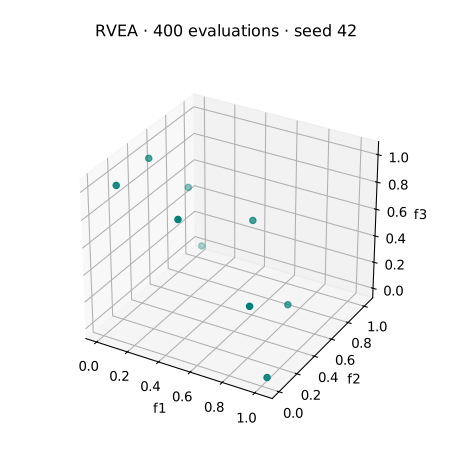
Measured with VAMOS 1.4.0; the observations and provenance retain the inputs and results.
Understand the configuration
| Setting | Meaning in this example |
|---|---|
n_partitions(3) |
A three-objective simplex lattice has comb(3 + 3 - 1, 3 - 1) = 10 vectors. |
| Population 10 | Matches the reference-vector count exactly. Arbitrary incompatible values fail. |
alpha(2.0) |
Controls the progression of the angle penalty. |
adapt_freq(0.1) |
Configures reference-vector adaptation frequency. |
Numeric mutation probability 1/12 |
One over the 12 variables, written as a number. |
VAMOS 1.2.0: RVEA and AGE-MOEA resolve "1/n" like the other algorithms, so prob="1/n" is equivalent to 1/12 here.
Development after 1.4.0: the population no longer has to be a lattice. reference_vectors(path=...) reads the vectors from a file, or from a directory of jMetal's W{n_obj}D_{pop_size}.dat files, as MOEA/D and NSGA-III do: with jMetal's W3D_100.dat, which VAMOS ships, RVEA runs 100 individuals with three objectives, from the same vectors as MOEA/D and NSGA-III given the same file. reference_vectors(divisions=H1, inner_divisions=H2) runs Deb and Jain's two-layer lattice, which gives usual population sizes with many objectives (156 with eight objectives, H1 = 3 and H2 = 2). See reference and weight vectors.
Interpret the result and its limits
Each X row aligns with the same F row. This lesson explicitly requests population mode, then computes the feasible non-dominated subset separately. All objectives are minimized. A non-dominated row is only non-dominated among the available rows; it need not be Pareto optimal. The retained observations contain the actual arrays and configuration.
Reference vectors are directions, not target solutions on the DTLZ2 unit sphere. Ten vectors give deliberately sparse coverage. This example enables feasibility handling, but its unconstrained problem does not exercise constraint survival. A finished budget is not evidence that the surface has been reached.
VAMOS 1.2.0: RVEA keeps one solution per reference vector that has any, the one with the smallest angle-penalized distance, as Cheng et al. [1], PlatEMO and pymoo do. Vectors without a solution leave the population, and the result, smaller than pop_size; the recorded run above returns 9 rows for its 10 vectors. Parents are drawn by random permutations of the population, as in pymoo (the article only says "random"). Two choices follow pymoo rather than the article: the angle penalty uses M = 1 with two objectives, and the ideal point accumulates across generations. VAMOS 1.1.0 filled the population up to pop_size with further solutions taken in vector order, which favoured the vectors listed first, those near (0, …, 0, 1), and drew parents with replacement.
VAMOS 1.2.0: with constraints, RVEA's survival keeps feasible solutions first. constraint_handling makes it judge feasibility and violation by one of jMetal's constraint-handling techniques: cdp, violated_constraints, epsilon_constrained or push_pull. See choose a constraint-handling technique.
This run has no constraints. Before using a constrained or discrete problem, check the capability matrix and constraint convention. Preserve complete runs through the canonical lifecycle; the teaching JSON is not a replay bundle.
Try one controlled change
Set partitions to 4 and compute the matching population with the same formula (15 for three objectives). Keep a common evaluation budget when comparing, record the changed direction set, and use repeated seeds.
Next: use T06 to turn this example into a reproducible comparison.
References
[1] Cheng, R., Jin, Y., Olhofer, M., and Sendhoff, B. (2016). A Reference Vector Guided Evolutionary Algorithm for Many-Objective Optimization. IEEE Transactions on Evolutionary Computation, 20(5), 773–791. DOI: 10.1109/TEVC.2016.2519378.